Scientific Python (NumPy, SciPy, & pandas)

4. Scientific Python (NumPy, SciPy, & pandas)#

Python has two large communities: web development and scientific computing. Each group has a few core packages that they add on top of base python. In this section, we will

4.1. NumPy#

The first package we will add to python is NumPy. To install numpy, type conda install numpy or pip install numpy depending on what package manager you are using.

I then recommend reading the NumPy beginners guide at https://numpy.org/doc/stable/user/absolute_beginners.html. I will only be able to summarize it here.

4.1.1. Importing NumPy#

import numpy as np

We use the python keyword import to bring numpy into our namespace. However, we rename it to np because we are lazy. Using np is a convention.

4.1.2. What is NumPy?#

4.1.3. Array basics#

a = np.array([1,  2,  3,  4,  5,  6,  7,  8,  9, 10])

4.1.3.1. Slicing#

data = np.array([1, 2, 3])
data[1]
data[0:2]
data[1:]
data[-2:]

NumPy Indexing

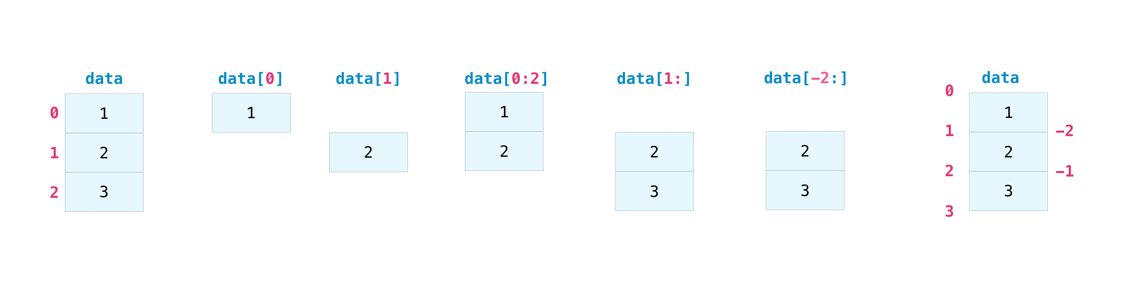
Note that in the above image it does not clearly show that data[0] and data[1] return the scalar value at those indices and not an array. However, data[:0] will slice data and return a one element array [1].

Important

Do not use np.append() if possible. and especially inside loops. NumPy arrays are similar to C-arrays, so all objects are next to eachother in memory. Therefore, appending to a numpy array needs to copy the entire array. Doing this once is ok, doing this inside a loop can take a lot of time.

This is not a feature of Python lists. Therefore, if you need to build up an array, do it as a list then convert it to an array.

4.1.3.2. 1D vs 2D#

>>> a = np.array([1, 2, 3, 4, 5, 6, 7])
>>> a.shape
(7,)
>>> a
array([1, 2, 3, 4, 5, 6, 7])
>>> a.T
array([1, 2, 3, 4, 5, 6, 7])
>>> a.T.shape
(7,)
>>> a = a[:, np.newaxis]
>>> a
array([[1],
       [2],
       [3],
       [4],
       [5],
       [6],
       [7]])
>>> a.shape
(7, 1)
>>> a.T.shape
(1,7)

In 2D arrays, the axis are (row, column).

4.1.3.3. Copies vs Views#

NumPy uses both copies and views.

x = np.array([1,2,3])
z = x
print(z is a)
print(x, z)
z[1] = 5
print(z is a)
print(x, z)

Learn to use copy() when needed.

4.1.3.4. Arrays vs Lists#

a * 2

What if a = np.array([1, 2, 3]) vs a = [1, 2, 3]? In NumPy this is called broadcasting.

np.zeros, np.ones.

Note

If you know the size of your final array, use np.zeros or np.empty then fill the array indexes with values. This is significantly faster than using np.append.

4.1.4. Random numbers#

One of the most used features in NumPy is getting random numbers. NumPy has an excellent tutorial, but note, NumPy had a major change to how you should create random numbers in

https://realpython.com/numpy-random-number-generator/

import numpy as np
rng = np.random.default_rng()

rng.uniform()
rng.uniform(low=3.4, high=5.6)
rng.integers(3)
rng.random(size=(5,))
rng.random(size=(3, 4, 2))
rng.standard_normal(size=(5,1))

.random returns random floats in the half-open interval [0.0, 1.0).

Note

What if I need to get the same random number the next time I run my code? Use a seed when setting up your random generator rng = np.random.default_rng(12345).

4.2. SciPy#

SciPy has a lot of useful features. We will predominately use it optimize and stats modules. However, you may need its Fourier transforms, numerical integration methods, interpolations, Linear Algebra, image processing, and signal processing modules.

4.2.1. scipy.optimize#

The scipy.optimize.minimize function minimizes a functions, given as starting set of values (x0) and a few options docs, tutorial.

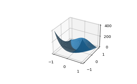
Lets look at fitting a built-in SciPy function, the Rosenbrock.

sum(100.0*(x[1:] - x[:-1]**2.0)**2.0 + (1 - x[:-1])**2.0)

Rosenbrock Function

>>> from scipy.optimize import minimize, rosen
>>> x0 = [1.3, 0.7, 0.8, 1.9, 1.2]
>>> res = minimize(rosen, x0, method='Nelder-Mead', tol=1e-6)
>>> res.x
array([ 1.,  1.,  1.,  1.,  1.])

We can also look at bounded and constrained minimizations tutorial.

fun = lambda x: (x[0] - 1)**2 + (x[1] - 2.5)**2

cons = ({'type': 'ineq', 'fun': lambda x:  x[0] - 2 * x[1] + 2},
 {'type': 'ineq', 'fun': lambda x: -x[0] - 2 * x[1] + 6},
 {'type': 'ineq', 'fun': lambda x: -x[0] + 2 * x[1] + 2})
 
bnds = ((0, None), (0, None))

res = minimize(fun, (2, 0), method='SLSQP', bounds=bnds, constraints=cons)
res.x

4.2.2. scipy.stats#

From the SciPy documentation:

This module contains a large number of probability distributions, summary and frequency statistics, correlation functions and statistical tests, masked statistics, kernel density estimation, quasi-Monte Carlo functionality, and more.

Statistics is a very large area, and there are topics that are out of scope for SciPy and are covered by other packages. Some of the most important ones are:

statsmodels: regression, linear models, time series analysis, extensions to topics also covered by scipy.stats.

Pandas: tabular data, time series functionality, interfaces to other statistical languages.

PyMC: Bayesian statistical modeling, probabilistic machine learning.

scikit-learn: classification, regression, model selection.

Seaborn: statistical data visualization.

rpy2: Python to R bridge.

We will be covering all of these other packages later in the semester.

We will use three subsections of scipy.stats:

scipy.stats has a lot of discrete, continuous, and multivalent distributions. This adds to NumPy with distributions such as an exponentially modified Normal, a Half-Cauchy, a power law, a Laplace, multivariate_normal, a Special Orthogonal matrix (SO(N)), a Poisson discrete, and a binomial discrete.
scipy.stats has advanced summary statistics such as moments, trimmed mean, kurtosis, and weighted geometric mean. It can even computer a binned statistic for one or more sets of data.
And it even has the functions we need for Hypothesis testing (week 4).

from scipy.stats import lognormal, skew

4.3. pandas#

pandas is a package for working with tabular data. Above we asked if NumPy 2D arrays were (row, column) vs (column, row). For tabular data specifically, it should be assign the axes to observations and variables.

pandas has a great “10 minutes to pandas” tutorial. Read this tutorial.

4.4. Tidy Data#

Tidy data is a framework to structure data in a way that simplifies the analysis. The full details can be seen at https://tidyr.tidyverse.org/articles/tidy-data.html.

Most datasets are made up of rows and columns. Tidy data is a formalism of mapping meaning to a data set’s structure. A data set is messy or tidy depending on how rows, columns and tables are matched up with observations, variables and types. In tidy data:

Each variable is a column; each column is a variable.
Each observation is a row; each row is an observation.
Each value is a cell; each cell is a single value.

Note

The definition of “value” can sometimes mean more than one number. For exmaple, is the spectral flux a sinlge value or should the value be a key that points to a new table that contains the spectra?

The five most common problems in data sets are:

Column headers are values, not variable names.
Multiple variables are stored in one column.
Variables are stored in both rows and columns.
Multiple types of observational units are stored in the same table.
A single observational unit is stored in multiple tables.

4.4.1. Example#

You may have a data set like this:

	treatment_a	treatment_b
John Smith	NA	2
Jane Doe	16	11
Mary Johnson	3	1

You can see that variables are stored in both rows and columns. Flipping the rows and columns don’t make it any better. You can see that values (either numbers or stings) are in every cell, including the headers.

4.5. Reading in data#

4.5.1. pandas#

For the most part, you will use pandas.read_csv.

pd.read_csv('data.csv')

pandas also has readers and writers for Excel files, Python pickle objects, xml, latex, hdf5, sql, and more.

4.5.2. NumPy#

NumPy works well, but does not give you the tabular data specific resources that you can find in pandas.

numpy.genfromtxt('data.csv', delimiter=',')

4.5.3. Python#

Only do this if you need to read in text and not a data set, or for some reason you need to build your own parser. But please, do your best to not build your own parser.

# Open the file in read mode
file = open("geeks.txt", "r")
# Read the entire content of the file
content = file.read()
# Print the content
print(content)
# Close the file
file.close()

4.6. Suggested Reading#

Vasiliev “Python For Data Science” chapter 3 “Python Data Science Libraries”
Vasiliev “Python For Data Science” chapter 4 “Accessing Data From Files and APIs”
https://numpy.org/doc/stable/user/absolute_beginners.html
https://numpy.org/doc/stable/reference/random/index.html
https://realpython.com/numpy-random-number-generator/
https://www.w3schools.com/python/scipy/index.php
https://docs.scipy.org/doc/scipy/tutorial/optimize.html#local-minimization-of-multivariate-scalar-functions-minimize
https://docs.scipy.org/doc/scipy/tutorial/optimize.html#bounded-minimization-method-bounded
https://pandas.pydata.org/pandas-docs/stable/user_guide/10min.html
https://www.w3schools.com/python/pandas/default.asp
https://colab.research.google.com/notebooks/mlcc/intro_to_pandas.ipynb
https://tidyr.tidyverse.org/articles/tidy-data.html
https://vita.had.co.nz/papers/tidy-data.html

Scientific Python (NumPy, SciPy, & pandas)

Contents

4. Scientific Python (NumPy, SciPy, & pandas)#

4.1. NumPy#

4.1.1. Importing NumPy#

4.1.2. What is NumPy?#

4.1.3. Array basics#

4.1.3.1. Slicing#

4.1.3.2. 1D vs 2D#

4.1.3.3. Copies vs Views#

4.1.3.4. Arrays vs Lists#

4.1.4. Random numbers#

4.2. SciPy#

4.2.1. scipy.optimize#

4.2.2. scipy.stats#

4.3. pandas#

4.4. Tidy Data#

4.4.1. Example#

4.5. Reading in data#

4.5.1. pandas#

4.5.2. NumPy#

4.5.3. Python#

4.6. Suggested Reading#