
12. Dimensionality Reduction (PCA)#
12.1. Principal component analysis (PCA)#
(Monday)
The theory of PCA just the theory of rotation in linear algebra. When I understood PCA, I finally understood Quantum Mechanics.
12.1.1. Cover Robinson 4.6.#
Covariance & PCA
12.1.2. Method:#
Standardize data
Find correlations
Find principal components
Transform Data
12.1.3. Advantages and Disadvantages of Principal Component Analysis#
(from https://www.geeksforgeeks.org/principal-component-analysis-pca/)
Advantages
Multicollinearity Handling: Creates new, uncorrelated variables to address issues when original features are highly correlated.
Noise Reduction: Eliminates components with low variance (assumed to be noise), enhancing data clarity.
Data Compression: Represents data with fewer components, reducing storage needs and speeding up processing.
Outlier Detection: Identifies unusual data points by showing which ones deviate significantly in the reduced space.
Disadvantages of Principal Component Analysis
Disadvantages
Interpretation Challenges: The new components are combinations of original variables, which can be hard to explain.
Data Scaling Sensitivity: Requires proper scaling of data before application, or results may be misleading.
Information Loss: Reducing dimensions may lose some important information if too few components are kept.
Assumption of Linearity: Works best when relationships between variables are linear, and may struggle with non-linear data.
Computational Complexity: Can be slow and resource-intensive on very large datasets.
Risk of Overfitting: Using too many components or working with a small dataset might lead to models that don’t generalize well.
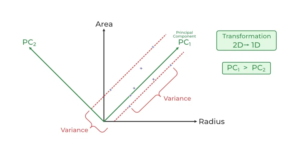
12.1.4. Dimensional Reduction#
12.1.5. PCA in Python#
(Wednesday)
(Example from https://www.geeksforgeeks.org/principal-component-analysis-pca/)
import pandas as pd
import numpy as np

# Here we are using inbuilt dataset of scikit learn
from sklearn.datasets import load_breast_cancer

# instantiating
cancer = load_breast_cancer(as_frame=True)
# creating dataframe
df = cancer.frame

# checking shape
print('Original Dataframe shape :',df.shape)

# Input features
X = df[cancer['feature_names']]
print('Inputs Dataframe shape   :', X.shape)
# Standardization
X_mean = X.mean()
X_std = X.std()
Z = (X - X_mean) / X_std
# covariance
c = Z.cov()

# Plot the covariance matrix
import matplotlib.pyplot as plt
import seaborn as sns
sns.heatmap(c)
plt.show()
eigenvalues, eigenvectors = np.linalg.eig(c)
print('Eigen values:\n', eigenvalues)
print('Eigen values Shape:', eigenvalues.shape)
print('Eigen Vector Shape:', eigenvectors.shape)
# Index the eigenvalues in descending order
idx = eigenvalues.argsort()[::-1]

# Sort the eigenvalues in descending order
eigenvalues = eigenvalues[idx]

# sort the corresponding eigenvectors accordingly
eigenvectors = eigenvectors[:,idx]

explained_var = np.cumsum(eigenvalues) / np.sum(eigenvalues)
explained_var
n_components = np.argmax(explained_var >= 0.50) + 1
n_components
# PCA component or unit matrix
u = eigenvectors[:,:n_components]
pca_component = pd.DataFrame(u,
                             index = cancer['feature_names'],
                             columns = ['PC1','PC2']
                            )

# plotting heatmap
plt.figure(figsize =(5, 7))
sns.heatmap(pca_component)
plt.title('PCA Component')
plt.show()
# Matrix multiplication or dot Product
Z_pca = Z @ pca_component
# Rename the columns name
Z_pca.rename({'PC1': 'PCA1', 'PC2': 'PCA2'}, axis=1, inplace=True)
# Print the  Pricipal Component values
print(Z_pca)
or
from sklearn.decomposition import PCA

pca = PCA(n_components=2)  # Can be any size
pca.fit(Z)  # still need to scale data.
x_pca = pca.transform(Z)

# Create the dataframe
df_pca1 = pd.DataFrame(x_pca,
                       columns=['PC{}'.
                       format(i+1)
                        for i in range(n_components)])
print(df_pca1)
plt.figure(figsize=(8, 6))

plt.scatter(x_pca[:, 0], x_pca[:, 1],
            c=cancer['target'],
            cmap='plasma')

plt.xlabel('First Principal Component')
plt.ylabel('Second Principal Component')
plt.show()
12.1.6. PCA in R#
Not this year.
12.2. Alternatives to PCA#
(Friday)
PCA benefits and draw backs:
Pros:
Dimensionality Reduction: PCA effectively reduces the number of features, which is beneficial for models that suffer from the curse of dimensionality.
Feature Independence: Principal components are orthogonal (uncorrelated), meaning they capture independent information, simplifying the interpretation of the reduced features.
Noise Reduction: PCA can help reduce noise by focusing on the components that explain the most significant variance in the data.
Visualization: The reduced-dimensional data can be visualized, aiding in understanding the underlying structure and patterns.
Cons:
Loss of Interpretability: Interpretability of the original features may be lost in the transformed space, as principal components are linear combinations of the original features.
Assumption of Linearity: PCA assumes that the relationships between variables are linear, which may not be true in all cases.
Sensitive to Scaling: PCA is sensitive to the scale of the features, so standardization is often required.
Outliers Impact Results: Outliers can significantly impact the results of PCA, as it focuses on capturing the maximum variance, which may be influenced by extreme values.
When to Use:
High-Dimensional Data: PCA is particularly useful when dealing with datasets with a large number of features to mitigate the curse of dimensionality.
Collinear Features: When features are highly correlated, PCA can be effective in capturing the shared information and representing it with fewer components.
Visualization: PCA is beneficial when visualizing high-dimensional data is challenging. It projects data into a lower-dimensional space that can be easily visualized.
Linear Relationships: When the relationships between variables are mostly linear, PCA is a suitable technique.
https://elitedatascience.com/dimensionality-reduction-algorithms https://medium.com/nerd-for-tech/dimensionality-reduction-techniques-pca-lca-and-svd-f2a56b097f7c
https://medium.com/nerd-for-tech/dimensionality-reduction-techniques-pca-lca-and-svd-f2a56b097f7c
Note
For science the two main issues of PCA are the lack of propagating uncertainties and the inherent linear assumptions.
12.2.1. Incorporating Uncertainties#
The main issue with PCA in science is that it does not account for uncertainties in the measurements.
https://iopscience.iop.org/article/10.3847/1538-4357/aaec7e/pdf
SNEMO uses Expectation Maximization Factor Analysis (EMFA)
https://scikit-learn.org/stable/modules/generated/sklearn.decomposition.FactorAnalysis.html
12.2.2. Doing nonlinear dimensionality reduction#
Also, PCA is inherently linear. With infinitely many PCA features you can shift a spectral line, or you can do a non-linear dimensionality reduction and represent a spectral line shift by a single parameter.